Probability
The Analysis of Data, volume 1
Basic Combinatorics for Probability
$
\def\P{\mathsf{P}}
\def\R{\mathbb{R}}
\def\c{\,|\,}
$
1.6. Basic Combinatorics for Probability Spaces
Some knowledge of combinatorics is essential for probability. For example, computing the probability $\P(E)$ in the classical model on finite sample spaces $\P(E)=|E|/|\Omega|$ is equivalent to the combinatorial problem of enumerating the elements in $E$ and $\Omega$.
In the case of a two-stage experiment where stage 1 has $k$ outcomes and stage 2 has $l$ outcomes and every combination of results in the two stages is possible, the total number of combinations of results of stage 1 and 2 is $k\cdot l$. A formal generalization appears below.
Definition 1.6.1.
A $k$-tuple over the sets $S_1,\ldots,S_k$ is a finite ordered sequence $(s_1,\ldots,s_k)$ such that $s_i\in S_i$.
Proposition 1.6.1.
There are $\prod_{j=1}^k |S_j|$ ways to form $k$-tuples over the finite sets $S_1,\ldots,S_k$. In particular if $S_1=\cdots=S_k=S$ there are $|S|^k$ possible $k$-tuples.
Proof.
A $k$-tuple is characterized by picking one element from each group. There are $n_1$ elements in group 1, $n_2$ in group 2, and so on. Since choices in one group do not constrain the choices in other groups, the number of possible choices is $\prod_{j=1}^k |S_j|$.
Example 1.6.1.
The R code below generates all possible 3-tuples over $S_1=\{1,2\}$, $S_2=\{1,2,3\}$, and $S_3=\{1,2\}$. There are $2\cdot 3\cdot 2=12$ such possibilities.
expand.grid(S1 = 1:2, S2 = 1:3, S3 = 1:2)
##    S1 S2 S3
## 1   1  1  1
## 2   2  1  1
## 3   1  2  1
## 4   2  2  1
## 5   1  3  1
## 6   2  3  1
## 7   1  1  2
## 8   2  1  2
## 9   1  2  2
## 10  2  2  2
## 11  1  3  2
## 12  2  3  2
Definition 1.6.2.
Assuming that $n$ is a positive integer and $r\leq n$ is another positive integer, we use the following notation:
\begin{align*}
n!&= n\cdot (n-1)\cdot (n-2)\cdots 2 \cdot 1\\
(n)_r &= \frac{n!}{(n-r)!}\\
\begin{pmatrix}n\\r\end{pmatrix}& = \frac{(n)_r}{r!}=\frac{n!}{r!(n-r)!}.
\end{align*}
We refer to the function $f(n)=n!$ as the factorial function and to $\begin{pmatrix}n\\r\end{pmatrix}$ as $n$-choose-$r$.
The factorial function grows very rapidly as $n\to\infty$. The R code below shows the considerable magnitude of $n!$ even for small $n$.
## [1]     1     2     6    24   120   720  5040
## [8] 40320
The following proposition shows that the growth rate of $n!$ is similar to the growth rate of $(n/e)^n$ (see Chapter B in the appendix for a definition of the limit notation below).
Proposition 1.6.2 (Stirling's Formula)
\[\lim_{n\to\infty} \frac{n!}{n^{n+1/2} e^{-n}}=\sqrt{2\pi}.\]
Proofs are available in (Feller, 1968) or (Rudin, 1976).
Proposition 1.6.3.
The factorial function grows faster than any exponential:
\[\lim_{n\to\infty} \frac{a^n}{n!}= 0 \qquad \text{for all } a > 0.\]
Proof.
Using
\begin{align*}
\lim_{n\to\infty} \frac{a^n}{n^{n+1/2} e^{-n}} =
\lim_{n\to\infty} \frac{1}{\sqrt{n}} \left(\frac{ae}{n} \right)^n = 0, \qquad a > 0,
\end{align*}
and Stirling's Theorem, we get
\begin{align}
\lim_{n\to\infty} \frac{a^n}{n!}=0, \qquad a > 0.
\end{align}
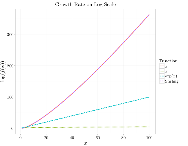
The proposition above is illustrated by the following graph comparing the growth rate on a log scale of the factorial with Stirling's approximation, an exponential function, and a linear function $x$. Stirling's approximation overlaps the factorial line indicating extremely good approximation.
x = 1:100
R = stack(list(`$x!$` = lfactorial(x), Stirling = log(2 *
    pi)/2 + (x + 1/2) * log(x) - x, `exp($x$)` = x,
    `$x$` = log(x)))
names(R) = c("lf", "Function")
R$x = x
qplot(x, lf, color = Function, lty = Function, geom = "line",
    xlab = "$x$", ylab = "$\\log(f(x))$", data = R,
    size = I(2), main = "Growth Rate on Log Scale")
Proposition 1.6.4.
The number of $r$-tuples over a finite set $S$ in which no element appears twice is $(|S|)_r$ and the number of different orderings of $n$ elements is $n!$.
Proof.
The first statement is a direct corollary of Proposition 1.6.1, where each value in the $r$ tuple is selected from the population of remaining or unselected items. The second statement follows from the first if $n=r=|S|$.
The following code generates all possible orderings of the letters a, b, and c. There are $3!=6$ such orderings.
library(gtools)
permutations(3, 3, letters[1:3])
##      [,1] [,2] [,3]
## [1,] "a"  "b"  "c"
## [2,] "a"  "c"  "b"
## [3,] "b"  "a"  "c"
## [4,] "b"  "c"  "a"
## [5,] "c"  "a"  "b"
## [6,] "c"  "b"  "a"
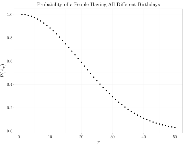
Example 1.6.2 (The Birthday Paradox).
There are $365^r$ possible assignments of birthdays to $r$ people. Using the previous proposition, the number of assignments of birthdays to $r$ people, assuming that all birthdays are different, is $(365)_r$. Under the classical probability model, the probability $\P(A_r)$ that a group of $r$ people will have all different birthdays is
\[\P(A_r)=\frac{|A_r|}{|\Omega|}=\frac{(365)_r}{365^r}.\]
For example, $\P(A_{30})\approx 0.294$, implying that it is likely to find recurring birthdays in a group of 30 people. The graph below shows how the probability of having different birthdays decays to zero as $r$ increases. The median (the value at which the probability is approximately 1/2) is $r=23$. The name "The Birthday Paradox" is sometimes associated with this example, since it is intuitively likely that 23 people will all have different birthdays with high probability.
r = 1:50
p = exp(lfactorial(365) - lfactorial(365 - r) - r *
    log(365))
qplot(main = "Probability of $r$ People Having All Different Birthdays",
    x = r, y = p, size = I(2), xlab = "$r$", ylab = "$P(A_r)$")
Proposition 1.6.5.
A population of $n$ elements has $\begin{pmatrix}n\\r\end{pmatrix}$ different subsets of size $r$. Equivalently there are $\begin{pmatrix}n\\r\end{pmatrix}$ ways to select $r$ elements out of $n$ distinct elements with no element appearing twice (selection without replacement) if order is neglected.
Proof.
There are $(n)_r$ ways to select $r$ elements out of $n$ elements if ordering matters (number of $r$-tuples over $n$ elements). Since there are $r!$ possible orderings of the selected values, the number we are interested in times $r!$ equals $(n)_r$. Dividing $(n)_r$ by $r!$ completes the proof.
Example 1.6.3.
We use R below to enumerate all possible subsets of size 3 out of a set of size 4. There are ten columns listing these subsets in accordance with $\begin{pmatrix}5\\3\end{pmatrix}=20/2$.
##      [,1] [,2] [,3] [,4] [,5] [,6] [,7] [,8] [,9]
## [1,] "a"  "a"  "a"  "a"  "a"  "a"  "b"  "b"  "b"
## [2,] "b"  "b"  "b"  "c"  "c"  "d"  "c"  "c"  "d"
## [3,] "c"  "d"  "e"  "d"  "e"  "e"  "d"  "e"  "e"
##      [,10]
## [1,] "c"
## [2,] "d"
## [3,] "e"
Example 1.6.4.
In poker, a hand is a subset of 5 cards (order does not matter) out of 52 distinct cards. The cards have face values (1-13) and suits (clubs, spades, hearts, diamonds). There are $|\Omega|=\begin{pmatrix}52\\5\end{pmatrix}$ different hands at poker since this is the number of subsets of size 5 from the 52 distinct cards. The probability that a random hand has five different face values under the classical model is \[4^5 \begin{pmatrix}13\\5\end{pmatrix}/\begin{pmatrix}52\\5\end{pmatrix}\approx 0.507\] as face values are chosen in $\begin{pmatrix}13\\5\end{pmatrix}$ ways and there are four suits possible for each of the five face values.
Example 1.6.5.
The number of sequences of length $p+q$ containing $p$ zeros and $q$ ones is $\begin{pmatrix}p+q\\p\end{pmatrix}$ (choosing $p$ among $p+q$ sequence positions and assigning them to zero values causes the remaining positions to be automatically assigned to one values).
Example 1.6.6.
Assuming that the U.S. Senate has 60 male senators and 40 female senators, the probability under the classical probability model of selecting an all-male committee of 3 senators is
\begin{align*}
\P(E) &= \frac{|E|}{|\Omega|}=
\frac{\text{number of samples of 3 out of 60 without
order and replacement}}{\text{number of samples of 3 out
of 100 without order and replacement}}\\
&= \frac{\left(
\begin{array}{c}
60 \\
3 \\
\end{array}
\right)}{\left(\begin{array}{c}
100 \\
3 \\
\end{array}
\right)}=\frac{60\cdot 59\cdot 58}{3\cdot 2}\frac{3\cdot 2}{100\cdot
99\cdot 98}\approx 0.211.
\end{align*}
Intuitively, if the frequency of all male committees is significantly larger than 21%, we may conclude that the classical model is inappropriate.
Proposition 1.6.6 (Binomial Theorem)
\begin{align*}
(x+y)^n = \sum_{k=0}^n \begin{pmatrix}n\\k\end{pmatrix}x^{n-k}y^k.
\end{align*}
Proof.
Expanding the expression \[(x+y)^n=(x+y)(x+y)\cdots(x+y)\] we see that it contains many additive terms, each corresponding to a pick of $x$ or $y$ from each of the product terms above. Collecting equal additive terms $x^{n-k}y^{k}$ for $k=0,\ldots,n$ (the sum of the two exponents must be $n$) we have $\begin{pmatrix}n\\k\end{pmatrix}$ possible selections of $k$ choices of $y$ out of $n$ leading to the term $\begin{pmatrix}n\\k\end{pmatrix}x^{n-k}y^k$. Repeating this argument for all possible $k=0,\ldots,n$ completes the proof.
The description above corresponds to choosing $r$ elements out of $n$ distinct elements, or alternatively placing $n$ distinct elements into two bins --- one with $r$ elements and one with $n-r$ elements. A useful generalization is placing $n$ distinct elements in $k$ bins with $r_i$ elements being placed at bin $i$, for $i=1,\ldots,k$.
Proposition 1.6.7.
The number of ways to deposit $n$ distinct objects into $k$ bins with $r_i$ objects in bin $i$, $i=1,\ldots,k$, is $n!/(r_1!\cdots r_k!)$.
Proof.
Repeated use of the Proposition 1.6.5 shows that the number is
\[\begin{pmatrix}n\\r_1\end{pmatrix}\begin{pmatrix}n-r_1\\r_2\end{pmatrix}
\begin{pmatrix}n-r_1-r_2\\r_3\end{pmatrix} \cdots \begin{pmatrix}n-r_1-\cdots-r_{k-2}\\r_{k-1}\end{pmatrix}.\]
Canceling common factors in the numerators and denominators completes the proof.
Example 1.6.7.
A throw of twelve dice can result in $6^{12}$ different outcomes. The event $A$ that each face appears twice can occur in as many ways as twelve dice can be arranged in six groups of two each. Assuming the classical probability model, the above proposition implies that
\[\P(A)=\frac{|A|}{|\Omega|}=\frac{12!/(2^6)}{6^{12}} \approx 0.0034.\]
The following inequality is useful in bounding the probability of complex events in terms of the probability of multiple simpler events.
Proposition 1.6.8. (Boole's Inequality)
For a finite or countably infinite set of events $A_i$, $i\in C$
\begin{align*}
\P\left(\bigcup_{i\in C} A_i\right) \leq \sum_{i\in C} \P(A_i).
\end{align*}
Proof.
For two events the proposition holds since $\P(A\cup B)=\P(A)+\P(B)-\P(A\cap B)$ (Principle of Inclusion-Exclusion). The case of a finite number of sets holds by induction. The case of a countably infinite number of sets follows from continuity of the measure function (see Chapter E.2).