1.3. The Classical Probability Model on Finite Spaces
In the classical interpretation of probability on finite sample spaces, the probabilities of all elementary events $\{\omega\}, \omega \in \Omega$, are equal. Since the probability function must satisfy $\P(\Omega)=1$ we have \[\P(\{\omega\})=|\Omega|^{-1}, \qquad \text{for all}\quad \omega\in\Omega.\] This implies that under the classical model on a finite $\Omega$, we have \[\P(E)=\frac{|E|}{|\Omega|}.\]
The R code below demonstrates the classical model and the resulting probabilities on a small $\Omega$.
Omega = set(1, 2, 3)
# all possible events
2^Omega
## {{}, {1}, {2}, {3}, {1, 2}, {1, 3}, {2, 3},
##  {1, 2, 3}}
# size of all possible events
sapply(2^Omega, length)
## [1] 0 1 1 1 2 2 2 3
# probabilities of all possible events under the
# classical model
sapply(2^Omega, length)/length(Omega)
## [1] 0.0000 0.3333 0.3333 0.3333 0.6667 0.6667
## [7] 0.6667 1.0000
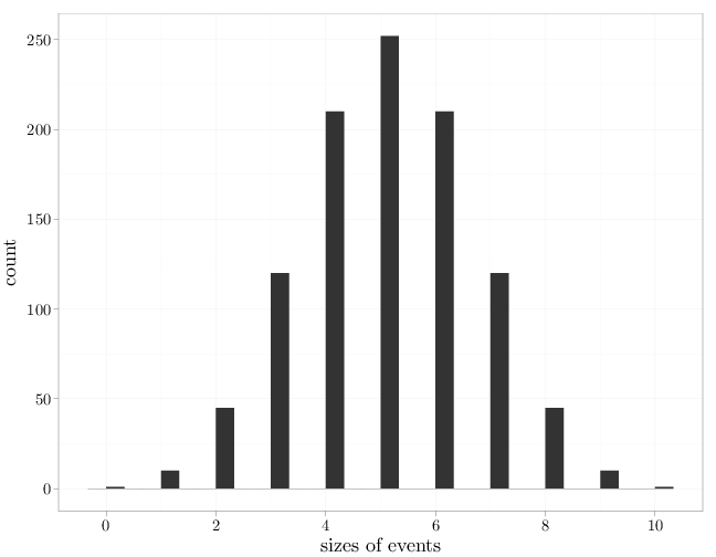
Note that the sequence of probabilities above does not sum to one since it contains probabilities of non-disjoint events. The R code below demonstrates this below for a larger set using by graphing the histogram of sizes and probabilities.
library(ggplot2)
Omega = set(1, 2, 3, 4, 5, 6, 7, 8, 9, 10)
# histogram of sizes of all possible events
qplot(sapply(2^Omega, length), xlab = "sizes of events")
# histogram of probabilities of all possible
# events under classical model
qplot(sapply(2^Omega, length)/length(Omega), xlab = "probability of events")

The left-most and right-most bars represent two sets with probabilities 0 and 1, respectively. These sets are obviously $\emptyset$ and $\Omega$.